White Paper
Bird’s Eye View on Tensilica Vision DSPs
August 2024
The increasing use of cameras in automotive advanced driver assistance systems (ADAS) has resulted in a greater demand for the capability and performance of vision applications. This demand requires sophisticated vision processing algorithms and powerful digital signal processors (DSPs) to run them. Because of the limited power and cost budgets of these embedded systems, it is important that the DSP’s instruction set architecture (ISA) is efficient and easy to program.
This paper overviews the Xtensa Bird’s Eye View (BEV) function version 1.0.0. The primary purpose of this paper is to examine the BEV or 360-degree view from a car. We mount four fish-eye cameras on a car's front, left, back, and right sides and input four fish-eye images to the BEV function. The BEV function will produce a bird’s eye view output. This bird’s eye view helps to see objects in the “blind spot,” parking in tight spaces, and is useful in ADAS applications. BEV also helps in driving heavy vehicles safely [11].
Overview
Introduction
A Bird’s Eye View (BEV) system for a car usually consists of four wide-angle fish-eye cameras with some overlap in the adjacent camera images. These cameras are mounted on the vehicle facing different directions, viz. front, left, back, and right, for a 3600 perception of the surrounding environment. The images from these four cameras are undistorted, and the top homographies are initially calculated during calibration. After calibration, high-quality surround-views can be synthesized at runtime. The BEV not only broadens the driver’s view to eliminate blind spots but is very helpful in parking in tight spaces, spotting pedestrians, and other related driving assistance tasks.
After being extrinsically calibrated, cameras in the BEV system should be fixed to keep the homographies unchanged. However, collisions, bumps, uneven road surfaces, or slopes may destroy the initial spatial structure of the camera system during calibration. If the initial homographies are still used and not properly adjusted, the generated surround views will have observable geometric misalignment. In such cases, promptly correcting the BEV’s homographies online is very important for driving safety.
The BEV function in this paper assumes that one-time homography calibration is already done and aims to correct the geometric misalignment online by adjusting the initial homographies to cope with current conditions.
The BEV function described in this paper is tested on Vision 240 DSP and Vision 341 DSP.
Modes
Calibration Mode
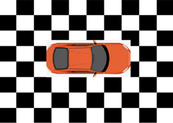
Figure 1 shows the calibration mode. In calibration mode, the car is parked on the “known” floor pattern (typically, a chessboard pattern or stripes pattern). The fish-eye camera input images are undistorted. Top homographies are calculated to find relations or transformations between four undistorted input images and the output BEV image. Reference scalar C code is available for automatic calibration—optimized Vision DSP functions are not supported.
Runtime Mode
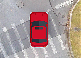
Figure 2 shows the runtime mode. Here, the car is on the road and in an “unknown” surrounding. We apply fixed un-distortion and fixed homography transformation to generate an output image in the runtime mode. If correction is enabled, the BEV function will correct the geometric misalignment online by adjusting the calibrated homographies. It can render the BEV output with or without these geometric misalignment corrections.
Bird’s Eye View Processing
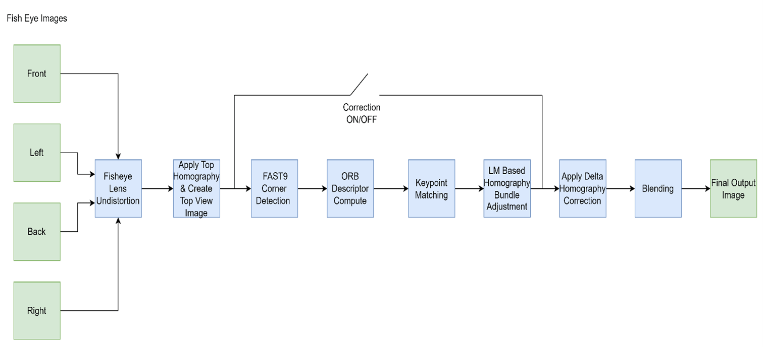
Figure 3 shows the BEV block diagram. The BEV accepts four fish-eye images from four cameras mounted on the car's front, left, back, and right sides. The top-view function undistorts the fish-eye images and uses top-homography matrices from calibration to create four top-view images viz Front-top, Left-top, Back-top, and Right-top. These four top-view images are stitched together and blended to create a final bird’s eye view output image. If correction is enabled, the key-points/corners are detected using the FAST9 algorithm in the overlapping areas, and matched pairs are identified using ORB descriptors. The Levenberg Marquardt-based bundle adjustment is run on these matched pairs to reduce errors between these matched pairs from all overlapping areas simultaneously and obtain the required homography correction. This correction is applied to provide a corrected output image. The following sections explain fish-eye lens un-distortion, homography, key-point detection, descriptor compute, key-point matching, bundle adjustment, and blending.
Fish-eye Lens Un-distortion
OpenCV provides a built-in function for fish-eye lens un-distortion [9][12], which uses the equidistant projection model to correct fish-eye distortion. The model assumes that the image is projected onto a sphere and that the distortion is caused by mapping the spherical coordinates to the image plane.
The following equation can represent the fish-eye lens distortion model:

where,
-
 xu and yu are the normalized coordinates of a point in the undistorted image
 - xd and yd are the normalized coordinates of the same point in the distorted image
- r is the radial distance from the center of the image to the point (xu,yu)
- k1, k2, k3, and k4 are the coefficients that describe the distortion of the fish-eye lens
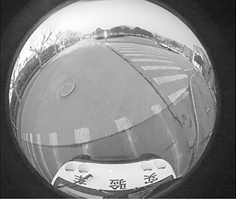
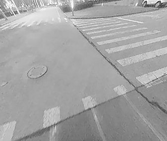
Figure 5 shows an undistorted image obtained from the fish-eye distorted image in Figure 4, using the above equations.
Homography
Refer to Figure 6 below. Homography is a transformation matrix that maps the same point on the common plane, which is the point (x, y) in one image plane of Camera 1 to the corresponding point (x’, y’) in another image plane of Camera 2 (up to a scale factor) as follows:

The homography matrix is a 3x3 matrix but with 8 degrees of freedom, as it is estimated up to a scale. It is generally normalized by assuming h33 = 1.0. Top homography matrices that relate key points in four un-distorted images to the output image are calculated during calibration mode and saved and applied during runtime mode.
![Points on the common plane, viewed on two image planes, are related by homography matrix H12 [8]](/content/dam/cadence-www/global/en_US/images/resources/whitepaper/birds-eye-view-on-tensilica-vision-dsps-wp-fig-6.png)
FAST9 Key-Point detection
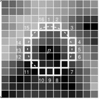
Key points in the image are points with significant intensity change. Key points and their locations can be found by different key-point detection algorithms such as FAST-9, SIFT, Harris corners, AKAZE, etc. We have used FAST-9 corner detection. It uses Down-Scale to create a pyramid of images, typically with a scale factor of 1.2. This allows it to produce multiscale features. The FAST-9 algorithm detects key points at different pyramid levels. FAST-9 extracts corners in the input by evaluating the pixels on the Bresenham circle of radius 4 around a candidate pixel – p (see Figure 7). If nine or more contiguous pixels are brighter than the candidate point at the center by at least a threshold value “t” or darker by at least “t,” then the candidate point “p” is considered a corner. Its strength is computed for each detected corner.
ORB Descriptor Compute
Once the key points or corners are detected, the neighborhood information of that key point is captured in a compact descriptor. There are different types of descriptors like Oriented and Rotated BRIEF (ORB), Scale Invariant Feature Transform (SIFT), Fast Retina Key-point (FREAK), etc. This implementation uses oriented and rotated BRIEF (ORB) descriptors. The ORB angle of every key point is calculated for rotation invariance. For that, it computes the intensity-weighted centroid of the patch with a detected corner at the center. The direction of the vector from this corner point to the centroid gives the orientation. The image patch around the key-point is effectively de-rotated by ORB angle for rotation invariance. Then, 256 comparisons are made around the key-point for a fixed set of pairs. If intensity-value1 is greater than intensity-value2, the bit is set for that pair, otherwise, the bit is reset to 0. Such 256 comparisons provide a 256-bit ORB descriptor for each key-point. Figure 8 shows the comparison of 256 fixed pairs to create the descriptor. Along with the descriptor, a 256-bit mask is created for each key-point. If the absolute difference in the above comparison is more than some threshold, the mask bit is set to 1; otherwise, it is reset to 0.
Key-Point Matching
Once we have the key-points identified and descriptors calculated for each key-point, we perform key-point matching between two images. This matching is done by comparing the key-point’s descriptors. For ORB descriptor matching, we perform the following steps:
For each key-point in Image1:
- For each key-point from Image2, the following conditions are checked:
- Does this key-point lie in the region of interest (i.e., it is present within ROI_X and ROI_Y)?
- Is the difference in pyramid levels less than levelDiffThreshold?
- Is the difference in ORB angle less than angleDiffThreshold?
- If the above conditions are satisfied, it then computes the hamming distance between two descriptors using:

where,
- desc1i and desc2i - ith bit of descriptor-1 and descriptor-2
- XOR - counts dissimilar bits between two inputs
- AND – looks for only non-trivial BRIEF differences of descriptor-1 and descriptor-2
- After repeating steps 1 and 2 for all descriptors in Image2, if the minimum hamming hdist is less than hamDistThreshold, the matched pair is stored.
Bundle Adjustment
If the same 3D world point on the road seen by two cameras does not overlap properly in the output, the final output will have artifacts. These artifacts are seen in the overlapping areas (highlighted by yellow color) along the diagonals of the output image. These artifacts include object contour lines not matching across two camera images, extra blurring or ghost images in the overlapping diagonal areas, etc. Many circumstances, such as improper calibration, uneven road surfaces, or cameras moving a little after calibration, etc., can cause such artifacts as homography matrices generated during calibration to need some correction to adjust to current modified conditions.
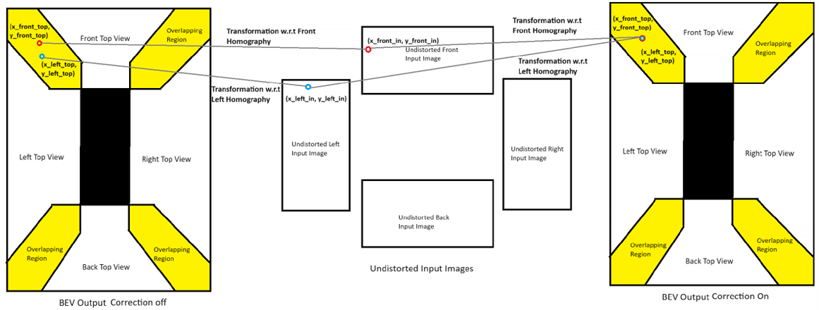
If homography correction is enabled, FAST-9 Corners are detected in the overlapping areas, and the corresponding ORB descriptors are computed with the help of the Cadence SLAM Library[4]. Using these descriptors, we perform matching in the overlapping areas. For example, as Figure 9 shows, if (x_front_top, y_front_top) corner from the front-top-view has found a matched pair at (x_left_top, y_left_top) in the left-top-view, then (x_front_top - x_left_top) and (y_front_top - y_left_top) gives an error in the matching pair. All such errors are accumulated for all the matched pairs in all four overlapping regions, and the overall error is minimized using the Levenberg Marquardt Method. Since all four overlapping areas are adjusted at once, this process is called “bundle adjustment.” The output of bundle adjustment is delta- homography-matrix, which provides the required homography adjustment. This homography adjustment is applied to get perfectly aligned output. Intensity blending is done in the overlapping areas so there are no visual artifacts in the final output.
Blending
Image blending is a popular technique in computer vision and image processing that allows us to combine two or more images to create a seamless and visually appealing result. Refer to [10], and as Figure 10 shows, two images can be blended together by giving weight α and (1-α) (where α ranges from 0.0 to 1.0) to input1 and input2 images.

![Blending two images [10]](/content/dam/cadence-www/global/en_US/images/resources/whitepaper/birds-eye-view-on-tensilica-vision-dsps-wp-fig-10.jpg)
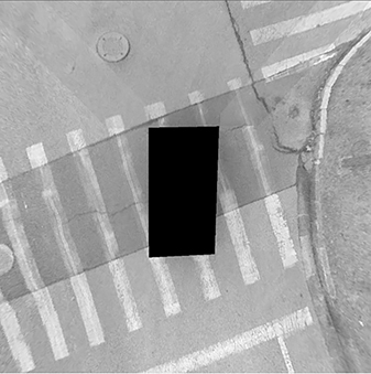
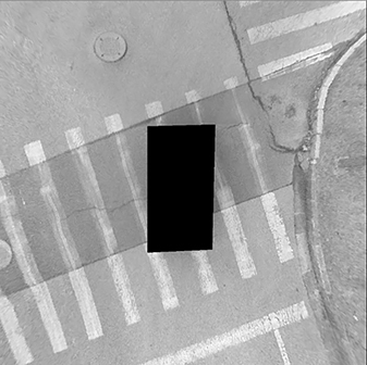
Figure 11 shows BEV output without blending. Intensity variations across diagonals of the image in the upper half of the image are very noticeable and annoying. Figure 12 shows BEV output with blending, which appears seamless and clean.
Results
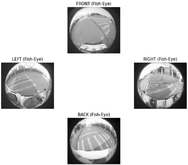
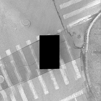
Figure 13 shows four fish-eye images as input to the BEV function. Figure 14 shows BEV output with correction OFF. In Figure 14, we can clearly see artifacts due to misalignment in all four overlapping regions, i.e., the diagonal regions of the image. Figure 15 shows the BEV output with correction ON. Figure 15 shows that even overlapping regions look great, as they are perfectly aligned using bundle adjustment-based correction. The BEV function also works with color (RGB) input images and produces color (RGB) output, as Figure 16 shows.
Reference Application
BEV function is currently implemented on:
- Vision 240 DSP
- Vision 341 DSP
A reference application that showcases the BEV function to generate a single output image of size 1000x1000 from four input fish-eye images of size 1280x1080 is available. The reference application also includes documentation, a user guide, and performance metrics.
Note:
- For detailed results, refer to the Xtensa Bird’s Eye View Function User’s Guide [5].
- For details on Vision 240 DSP, refer to [1]
- For details on Vision 341 DSP, refer to [2]
- For details on the Xtensa SLAM Library and Tile Manager, refer to [3] and [4] resp.
Summary
This paper presents an optimized implementation of the Bird’s Eye View functionality on the Vision 240 and Vision 341 DSPs. This function accepts four fish-eye camera images, viz. left, right, front, and back, as input and provides a bird’s eye view image output. In addition, if homography correction is enabled, online correction is provided without the need for re-calibration. Online homography correction corrects misalignments in the output using FAST9 key-point detection and ORB BRIEF descriptor-based matching, and the Levenberg Marquardt Bundle Adjustment method. Using this scheme, if the homographies of a calibrated surround-view system change moderately, the associated homographies can be corrected online. The achieved performance results show that the Cadence Tensilica DSPs with fixed and floating-point support are well-suited for this application.
Note: The current implementation of the BEV function on Vision DSPs is also available for color (RGB) images.
References
[1] Vision 240 DSP User’s Guide
[2] Vision 341 DSP User’s Guide
[3] Xtensa Vision Tile Manager Library User’s Guide
[4] Xtensa SLAM Application and SLAM Library User’s Guide
[5] Xtensa Bird’s Eye View Function User’s Guide
[6] Dataset Provided by: Tianjun Zhang, one of the writers of the paper “Online Correction of Camera Poses for the Surround-view System: A Sparse Direct Approach”
[7] Tianjun Zhang, Nlong Zhao, Ying Shen, Xuan Shao, Lin Zhang, and Yicong Zhou. 2021. ROECS: A Robust Semi-direct Pipeline Towards Online Extrinsics Correction of the Surround-view System. In Proceedings of the 29th ACM International Conference on Multimedia (MM ’21), October 20–24, 2021, Virtual Event, China. ACM, New York, NY, USA, 9 pages.
[8] http://csundergrad.science.uoit.ca/courses/cv-notes/notebooks/19-homography.html
[9] https://docs.opencv.org/4.x/db/d58/group__calib3d__fish-eye.html
[10] http://graphics.cs.cmu.edu/courses/15-463/2010_spring/Lectures/blending.pdf
[11] "BIRD’S-EYE VIEW VISION-SYSTEM FOR HEAVY VEHICLES WITH INTEGRATED HUMAN-DETECTION"
[12] Juho Kannala and Sami Brandt. A generic camera model and calibration method for conventional, wide-angle, and fish-eye lenses. IEEE transactions on pattern analysis and machine intelligence, 28:1335–40, 09 2006.
Additional Information
For additional information on the unique abilities and features of Cadence Tensilica processors, refer to ip.cadence.com.